A massive amount of spatial data is available through Esri REST APIs. It is a popular publishing format for federal, state, and county governments so many of these data fall within the public domain. At the time of writing, there are 7266 datasets published on data.gov, 3426 sets on data.gov.uk, and 859 on open.canada.ca all of which are available through Esri REST APIs. Another large set of Esri REST APIs can be found at European Environment Agency Discover Map Services.
Many of these data are also available for download via other formats such as Geodatabase, shape, and zipped files. An advantage of learning to use Esri REST services over these other formats is that a user may filter their data prior to storing it locally, limiting download size and required data cleaning/filtering. Users may also go on to implement use of these APIs within programs and scripts and know that they are using the most current data available. Another advantage of utilizing Esri REST platforms is that they are available to non Esri clients allowing users to avoid costly subscription fees surrounding ArcGIS and other Esri software. Throughout this tutorial, we will be exploring how to query, clean, and map spatial data describing administrative forest boundaries. These data are published by the U.S. Forest Service.
It may surprise you to learn that it is often more challenging to navigate to the Rest API than to query it, especially for new users. For the sake of making this tutorial applicable to other Esri REST APIs, we will go through the initial steps of locating these resources.
Let’s begin at the page for Forest Service Enterprise Data
You should see a pane titled Map Services which looks like the following:
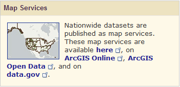
Click the ‘here’ hyperlink to go to a folder containing a collection of REST services published by the U.S. Forest Service. Feel free to browse around and explore all the available data sets here! When you are ready, select EDW/EDW_ForestSystemBoundaries_01 , which should be roughly a third of the way down. This will navigate you to the directory containing the data layers we want for this tutorial. If you’d like, you can select ArcGIS Online Map Viewer near the top of the page to further explore our data layers on a map. This is a great tool to explore the different fields within your data which will inform your query.
Moving forward, select the Administrative Forest Boundaries - National Extent (0) layer, then scroll to the bottom of the page and select Query. This will bring you to a page in which you can practice querying the REST API within the context of your browser. Each field you see here represents a parameter within a query URL made to the relevant API. This page is your friend. Seriously. If you’re attempting to implement the use of an Esri REST API within an R script it is extremely helpful to have a sterile and easy-to-read environment to play with different parameters in your query. We’ll begin querying via the ‘Where’ parameter. If you have any experience with SQL this should be fairly straightforward as the ‘Where’ parameter takes a SQL WHERE clause as it’s argument. If not, we will give you the tools you need to begin constructing simple WHERE clauses.
WHERE clauses are used to obtain an occurrence(s) within a data set where a certain field is equal to a given value. The general format is:
WHERE <field> = '<some value>'. In the context of this API the WHERE term is assumed, so we can leave that off.
Go ahead and enter:
FORESTNAME = 'Angeles National Forest'into the WHERE field.
Esri Rest queries, like SQL, are sensitive to the types of quotes one uses. Thus the above where statement works, however FORESTNAME = "Angeles National Forest" would return an error. If your queries are continually returning errors or empty values ensure you’re using single quotes and your capitalization is correct!
Enter an asterisk (*) into the Out Fields parameter. This indicates you wish to return all fields within the dataset. Hit Query (GET) at the bottom of the page and you should see some HTML describing an entry within the dataset appear at the base of your window. Hurray! You have successfully queried an Esri REST API!
Moving forward, let’s generalize this WHERE clause just a bit. For instance, let’s say you aren’t quite certain about the name of the national forest polygon you’re interested in obtaining. Or, better yet, let’s say you’re implementing this query within a program which takes in user input describing which national forest polygon to request, however you can’t depend on your users to enter a full or exact forest name. Try:
FORESTNAME LIKE '%Tahoe National%'This essentially makes a request to the API for an occurrence where the value within the FORESTNAME field contains the characters ‘Tahoe National’ potentially with other characters at the beginning or end. It is important to note that this parameter is still case sensitive.
Now that we’ve played with the query page just a bit, let’s begin to see how we might implement this in R.
If you haven’t already noticed, each time you hit Query (GET) the URL in the top of your browser updates. This is your query URL.
We will be using a few libraries within this tutorial for obtaining and viewing spatial data. If you don’t have the following packages you should install them via install.packages('') before proceeding.
library(sf)
library(leaflet)
library(geojsonsf)
library(dplyr)
library(urltools)
Change the Format field at the bottom of your page to GeoJSON and make another query. This time you should be redirected to a page containing the GeoJSON file describing the output from your query. GeoJSON is a simple and lightweight file format based on JSON (JavaScript Object Notation) designed to represent spatial data alongside non-spatial features. GeoJSON and JSON objects are syntactically identical to the code one would use to create a JavaScript object.
Now that we have the location of the relevant GeoJSON file, copy the URL from the top of your page and pass it to geojson_sf().
forest <- geojson_sf("https://apps.fs.usda.gov/arcx/rest/services/EDW/EDW_ForestSystemBoundaries_01/MapServer/0/query?where=FORESTNAME+LIKE+%27%25Tahoe+National%25%27&text=&objectIds=&time=&geometry=&geometryType=esriGeometryEnvelope&inSR=&spatialRel=esriSpatialRelIntersects&relationParam=&outFields=*&returnGeometry=true&returnTrueCurves=false&maxAllowableOffset=&geometryPrecision=&outSR=&having=&returnIdsOnly=false&returnCountOnly=false&orderByFields=&groupByFieldsForStatistics=&outStatistics=&returnZ=false&returnM=false&gdbVersion=&historicMoment=&returnDistinctValues=false&resultOffset=&resultRecordCount=&queryByDistance=&returnExtentOnly=false&datumTransformation=¶meterValues=&rangeValues=&quantizationParameters=&featureEncoding=esriDefault&f=geojson")It should be noted that this code may generate a warning message stating ‘incomplete final line found.’ This is a result of the geojson file missing an end of file marker or a return at its end. This warning can safely be ignored in the context of this tutorial.
Let’s take a look at this data!
leaflet() %>%
  addProviderTiles("Esri.WorldStreetMap") %>%
addPolygons(data=forest, weight=2, color="blue")#derive bounding box and convert it to Polygon so we can plot it
bboxPoly <- st_bbox(forest) %>%
st_as_sfc()
leaflet() %>%
addProviderTiles("Esri.WorldStreetMap") %>%
addPolygons(data=forest, weight=2,color="blue") %>%
addPolygons(data=bboxPoly, weight=2, fill=FALSE, color="blue")#baseURL for Forest Service invasive species API
baseURL <- "https://apps.fs.usda.gov/arcx/rest/services/EDW/EDW_InvasiveSpecies_01/MapServer/0/query?"
#bounding box of tahoe national forest polygon
bbox <- st_bbox(forest)
#convert bounding box to character
bbox <- toString(bbox)
#encode for use within URL
bbox <- urltools::url_encode(bbox)
#EPSG code for coordinate reference system used by tahoe national forest polygon sf object
epsg <- st_crs(forest)$epsg
#set parameters for query
query <- urltools::param_set(baseURL,key="geometry", value=bbox) %>%
param_set(key="inSR", value=epsg) %>%
param_set(key="resultRecordCount", value=500) %>%
param_set(key="spatialRel", value="esriSpatialRelIntersects") %>%
param_set(key="f", value="geojson") %>%
param_set(key="outFields", value="*") %>%
param_set(key="geometryType", value="esriGeometryEnvelope") %>%
param_set(key="returnGeometry", value="true") %>%
param_set(key="returnTrueCurves", value="false") %>%
param_set(key="returnIdsOnly", value="false") %>%
param_set(key="returnCountOnly", value="false") %>%
param_set(key="returnZ", value="false") %>%
param_set(key="returnM", value="false") %>%
param_set(key="returnDistinctValues", value="false") %>%
param_set(key="returnExtentOnly", value="false") %>%
param_set(key="featureEncoding", value="esriDefault")
invasives <- geojson_sf(query)Let’s take a moment to look through the parameters of our query.
geometry
The first parameter is the input geometry, to which we pass the bounding box of the Tahoe National Forest. You’ll notice that before we pass the bounding box to the API we do a bit of formatting. First it is converted to the character class with the toString() function. We then pass it to url_encode(), because things like spaces and commas are represented within URLs with special ASCII character combinations.
inSR
We then set the input spatial reference. Here we are supplying the API with the coordinate reference system of our polygon. Without getting into too much detail, a coordinate reference system (commonly referred to as a CRS) is a reference point which provides context to coordinates (the coordinates of our bounding box in this case). The two main categories of coordinate reference systems are geographic and projected. Geographic systems are based on a spheroid and utilize angular units of measurement such as degrees of longitude or latitude. Projected systems are a spheroid projected onto 2-dimensional surface. EPSG:4326 and EPSG:3857 are two very common coordinate reference systems, the first being geographic and the latter being projected.
If you’re curious to learn more about coordinate reference systems an excellent explaination can be found here.
resultRecordCount
This parameter simply dictates how many observations we would like the API to return. The maximum number of records that can be returned is 1000, which is the default value for most REST APIs. The maximum value of records that can be returned is set by the server administrator. If we leave this field blank 1000 values will be returned, indicating that the number of requested records exceeds the maximum. Another indicator that the maximum number of records has been met is a boolean variable that will appear at the top of the requested GeoJSON page called exceededTransferLimit. If you would like to obtain a set of records within a given geometry which exceed the maximum, you should split your geometry over multiple requests, such that each individual input geometry contains less than the given maximum. (See Exercise 2 at the end of this document for more information)
spatialRel
Spatial relationship, given the value “esriSpatialRelIntersects” is stating that we want observations which intersect with the input geometry, which is the bounding box of our polygon in this case.
f
format is the file format in which our data will be returned.
outFields
This is the parameter which dictates which fields of the dataset will be returned. We pass an asterisk in order to get all fields. Alternatively if we just wanted the common name of the plant alongside its geometry we could pass ACCEPTED_COMMON_NAME to outFields.
We will not go into the remaining parameters, if you’d like to explore them yourself you can do so within the API reference.
The rest of parameters have been set at their default value. Note, if the default values of a parameter are being used their values do not need to be set within your query. For the purposes of this tutorial they were included to give a clear representation of parameters versus the base URL. The following (significantly smaller) chunk of code would accomplish the same goal. It should also be noted that esriSpatialRelIntersects is the default value of spatialRel.
#baseURL for  Forest Service invasive species API
baseURL <- "https://apps.fs.usda.gov/arcx/rest/services/EDW/EDW_InvasiveSpecies_01/MapServer/0/query?"
#bounding box of tahoe national forest polygon
bbox <- st_bbox(forest)
#convert bounding box to character
bbox <- toString(bbox)
#encode for use within URL
bbox <- urltools::url_encode(bbox)
#EPSG code for coordinate reference system used by tahoe national forest polygon sf object
epsg <- st_crs(forest)$epsg

#set parameters for query
query <- urltools::param_set(baseURL,key="geometry", value=bbox) %>%
  param_set(key="inSR", value=epsg) %>%
  param_set(key="resultRecordCount", value=500) %>%
  param_set(key="f", value="geojson") %>%
  param_set(key="outFields", value="*")
invasives <- geojson_sf(query)
Let’s take a look at our data!
leaflet() %>%
  addProviderTiles("Esri.WorldStreetMap") %>%
  addPolygons(data=forest, weight=2, color="blue") %>%
  addPolygons(data=invasives, weight=3, color="red")
Great! We have our invasive plant locations, as well as the boundaries to the Tahoe National Forest. Except, it seems that we have a decent number of invasive plant observations that don’t intersect the boundary of the national forest. If you remember, we passed a bounding box to the API, therefore we got all observations that intersected the bounding box rather than the polygon itself.
Let’s filter out all of the observations from the invasive plant API that don’t intersect the Tahoe National Forest polygon.
#spatially join invasives and forest
insideInvasives <- st_join(invasives,forest)
#remove na values (i.e. values where there is no spatial overlap)
insideInvasives <- na.omit(insideInvasives)
Note: the call to st_join() generates a message stating ‘although coordinates are longitude/latitude, st_intersects assumes that they are planar.’ This message was generated because we have passed an object which uses a geographic coordinate reference system to a function which assumes our data has been projected onto a 2-dimensional surface. In the context of this calculation the difference in results with a geographic versus projected CRS is negligible. However, if you are performing operations on data that spans an entire continent or is near either terrestial pole it can cause your calculations to return incorrect results. You should always carefully select your coordinate reference system prior to performing geographic calculations!
leaflet() %>%
  addProviderTiles("Esri.WorldStreetMap") %>%
  addPolygons(data=forest, weight=2, color="blue") %>%
  addPolygons(data=insideInvasives, weight=3, color="red")
And there you have it! We hope this tutorial has been informative!
Exercises: (Solutions available on github)
1. Use what you’ve learned throughout this tutorial to obtain and plot the major rivers of Spain.
These data can be located at the European Environment Agency Discover Map Services
Locate the European Countries API and the Hydrography API
Explore the available data layers within each API in the ArcGIS Online Map Viewer. Note: Ensure you select ArcGIS Online Mapviewer under ‘View in:’ not ‘View footprint in:’
Use the Contents pane in the left hand side of the mapviewer to toggle which data layers are shown
Hover your cursor over a layer name in the contents pane and select Show Table (small icon which looks like a data table) to view the data within that layer
Use the information you gather here to decide which data layers to utilize and how to construct your query
Query the European Countries API and obtain a polygon for Spain (Try to construct your query within R)
Use the returned data to derive and format a bounding box
Use the bounding box of Spain to query the Hydrography API to obtain the main rivers that intersect your bounding box.
Filter out all rivers that do not intersect Spain
create an interactive leaflet plot to display your data (Hint: The rivers are represented by Polyline objects so leaflet::addPolyLine() should be utilized to add them to your plot)
2. Obtain all observations of invasive plants within the Tahoe National Forest by splitting the bounding box into quarters and querying the Current Invasive Species Locations APIs for each individual quarter:
Derive the bounding box of the Tahoe National and convert it into a polygon with
st_as_sfc()Split the polygon into quarters with
st_make_grid(tahoeBox, n=2)Query the API for each quarter of the bounding box (bonus points if you can combine each of the returned sf objects into one)
Filter out observations that do not intersect the Tahoe National Forest
Make an interactive leaflet plot displaying the boundaries of the Tahoe National Forest, the quartered bounding box, and invasive locations within the Tahoe
We encourage you to compare your work to the exercise solutions which can be found on github.
References:
This tutorial was created in RStudio 1.2.5033 (RStudio Team, 2015), using R 3.6.2 (R Core Team, 2020) and RMarkdown 2.0 (J.J. Allaire, 2019).
We utilized two APIs, S_USA.InvasivePlantCurrent (Natural Resource Information Systems, U.S. Forest Service, 2020) and Administrative Forest (Automated Lands Program, U.S. Forest Service, 2020).
The following packages were used to obtain, clean, and visualize data:
sf (v0.9.2; Edzer Pebesma, 2020)
leaflet (v2.0.3; Joe Cheng, 2019)
geojsonsf (v1.3.3; David Cooley, 2020)
dplyr (v0.8.3; Hadley Wickham, 2019)
urltools (v1.7.3; Os Keyes, 2019)
Useful Links:
Coordinate Reference System and Spatial Projection (Leah Wasser, Earth Data Science, 2019)
API Meta data:
Resources:
Other Useful R Tools:
Thanks to Jason Jones on LinkedIn for providing a reference to Esri2sf, an R package designed to scrape features from ArcGIS Servers. This and many other R packages can be utilized to obtain data sets from specific sources.
Other useful packages include:
rgbif: Allows users to access to GBIF, a database of species occurrence records
dataRetrieval: Provides access to EPA water quality data
nhdplusTools: A set of tools to access and manipulate hydrographic
If you’d like to learn more, KDV offers R instruction through customized workshops and classes at Transmitting Science.
![]()